PUBLICATIONS RELATED 1950 Roscoe Giffin People of the PMS School District Part 2 (051-089)

Pine Mountain Settlement School
Series 18: PUBLICATIONS RELATED
Series 09: BIOGRAPHY
1950 Roscoe Giffin
People of the Pine Mountain School District,
Pine Mountain Community Study
Harlan County, Kentucky
PART 2 (051-089)

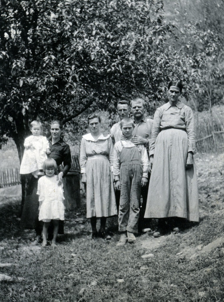
The Caldwell Family. mccullough_II_41b

TAGS: Roscoe Giffin, People of the Pine Mountain School District, Harlan County, Kentucky, Appalachian sociology, Appalachian culture, education, sociology of Eastern Kentucky,

PUBLICATIONS RELATED 1950 Roscoe Giffin People of the PMS School District Part 2 (051-089)

TRANSCRIPTION:
1950 Roscoe Giffin “People of the Pine Mountain School District, Harlan County, Kentucky”

p. 051

TABLE 14
HOUSEHOLDS DISTRIBUTED BY SIZE AND TYPE

p.052

TABLE 15
POPULATION DISTRIBUTED BY SIZE AND TYPE OF RESIDENT HOUSEHOLD

p.053

INCOME, ASSOCIATED VARIABLES, AND LEVELS OF LIVING

In a society which defines the family as that social unit in which shall rest the major responsibility for the welfare of individuals. It is important to have information as to the amounts. and sources of income available if we are to comprehend the levels of living which families and individuals achieve. This is a task of formulating the conceptual and statistical tools. Of measurement, a task shared commonly with all areas of scientific investigation. In. some realms of social life are tools of measurement are well developed in others we are plagued with all manner of difficulty and deficiencies. For example, we are able to make more quantitative statements about the families economic life than about the affectional. side of its activities. but as the. Presentation of our findings on the topics of this section developed. We shall have frequent reason to note that our economic data also are inadequate to answer with accuracy. Many of our questions in other. cases, we are limited simply to stating the questions thus. at the beginning the point is to be emphasized that our findings are in the Main Indicative rather than definitive as to the income, its sources and the resulting levels of living of the populations here studied.

It is hardly. Any longer a mark of economic sophistication to point out to the reader that in an exchange economy, there are at least two points of view from which the income position of a family must be considered. One is that of the amount of cash income received from the sale of the services of the employed persons, or from the sale of property. The other viewpoint requires a consideration. Of what goods and services it was possible for the family to acquire through the expenditure in the market place of its cash income. The second phase of the problem of income. Is closely identified with the question of the level of living which a family achieves. Although the concept of….

P.054

…”levels of living” Is more complicated by far than just a supply of purchasable. Goods and services it is. obvious that there is a very close and direct correlation present between the supply of money income and the supply of real income, and consequently the level of living.

In all households, the actual real income is greater than that can be purchased by its cash income. This follows from the obvious fact that in households there is much production resulting from the unpaid labor of its members, which adds to the stock of consumable goods and services. Thus, our study of income involves consideration not only of the position of the household and the exchange economy, but also as producer of goods and services to be consumed by its members. We must therefore add to our cash income some measure of the value of home or household production in our consideration of the types and distribution of income available to these families.

In order to formulate some tentative understandings of the causes of variation among the households in their supply of income, it will be necessary to study the income in relation to several variables. With which it is logically and quantitatively. Associated this will be. done both for money income and for our estimates of the money value of the household production.

p. 055

Cash Income: The basic data for the following description of the cash income of the households studied are shown in table 16. Households by neighborhoods and amount of cash income.

Information regarding the estimate of annual cash income for the year extending from July 1949 to July 1950 was obtained from 104 households. Here again, we must disavow any claim to being able to present anything more than data indicative of cash income. But since. all but a few obtained their cash from wage jobs with fairly well known rates of pay. And since most of the. Gross. Providing the information had a rather clear impression of the number of months during which the employed person had worked, It would seem reasonable to place considerable confidence in the data. Had we been dealing with a dominantly farm or business, enterprise group, particularly of the small scale type, the data would be probably less trustworthy. 1. difficulty with our data is that in order to allow for the inability of many. Persons to offer accurate figures. Those interviewed were asked simply to state their income in terms of the class interval shown in table 16. These intervals are so broad that detailed information of value was lost. With these preliminary cautions and explanations, we may turn to a simple presentation of the findings.

Cash income estimates ranged all the way from 17 cases less than $600 to five in excess of $4000. And since three of the last five are wage and salary earnings, it is probably true that they do not exceed $4000 by more than a few hundred dollars. The modal concentration was in the interval of $1500 to $2500 in which were 40 of the 104 households providing information.

p. 056

TABLE 16
HOUSEHOLDS BY NEIGHBORHOOD AND AMOUNT OF CASH INCOME

p.057

The mean or average cash income was $1810 for the 104 cases and a median estimate at $1725. The. generally low level of cash income can be brought out more forcefully if we compute the average for all cases providing information except those in excess of $4000. The average. then falls to three$1300. [1]

It is of some interest to notice the considerable differences Which exists among the various neighborhoods as regards cash income distribution.’ It is quite apparent, as will appear in several other ways, that these neighborhoods are distinguishable in more than name alone. in several cases, they appear to be rather distinct. sub-cultures within the general culture of the area.

The Pine Mountain and Isaacs Creek neighborhoods are apparently more prosperous, though less populous than the other neighborhoods these. neighborhoods are the most proximate to Pine Mountain School The lowest level of income was found along Greezy Creek below Big Laurel and approaching the Leslie County line. Here live several families of old age pensioners and several widows. Whose annual cash income seems little more than a pittance. The next lowest level of the income prevails in the extreme western portions of the new school district in the Incline neighborhood. The median of $1100. seems almost an overstatement to any one who has been in a number of the homes or observes the households with some care as he rides along the road in a car.In a number of cases, the low income recipients are families, not native to the area. They have come there as employees of several sawmill operations, but they have either….

[1.] The survey of Consumer Finance is sponsored by the Federal Reserve Board, reported a national main income per household in 1950 of $3520. Within the skilled in semi skilled occupational group, which is roughly comparable to the majority of an occupations covered in this study the mean income was.$3600 for. farm operators, the mean was $1900. Sources,: . Federal Reserve Bulletin. 1951 Survey of Consumer Finances. 2 pp. 921- 923.

p. 058

Not incapable of higher earnings or else the opportunities have not been available. Although the following comment probably should not be thought of as having any casual significance, it is of interest, nevertheless, to notice that neighborhoods of lowest income. Are those most distant from Pine Mountain School.

Value of Pome Production: If one studies carefully enough, the activities of a household, he will find there a little bit of almost everything that goes on in the exchange economy despite the fact that the home. Is no longer the core institution of our society. It is nevertheless true that within. it may yet be found those activities which are the primary function of the institution’s concerned with education. Religion, manufacturing, distribution, banking, recreation, medicine and health, et cetera, The home in recent years is being made the brunt. of no end of criticism for its failure to carry on these functions at a sufficient level of quantity and quality so as to meet the needs of its members and to thereby keep them from being “problems” For the school, law enforcement agencies psychiatrists, etc.

In the rather remote area Of this study, the home is perhaps less dependent upon other specialized institutions than is true of the urbanized areas of the country, whether they be in the country, Or city. We have attempted in this study to measure only a part of one Phase of these household activities and that is. The contribution its members make through direct production to the supply of consumable goods. There seems to be evidence to indicate that this measure may….

p. 059

Be well correlated with other activities which we are unable to describe quantitatively. This evidence will be submitted at the appropriate spot later in this presentation. For the present, we shall present our data on household production only.

In order to get an estimate of the amount of home produced foods are questionnaire included questions concerning the amounts of meat, fresh and canned fruits and vegetables, milk and dairy products. And eggs produced at home. In addition to these items, a question as to the coal and or wood produced on the land was included The quantities obtained from the preceding questions. Were then converted into dollar valuations by use of market price multipliers. As an example, pork was valued at an average price per pound of 40 cents. But a hog estimated to dress out at 200 pounds would represent home produced income. To the amount of $80? in order to measure the money value of the housing obtained by those who owned their home, a rental figure was imputed and Such cases. on the basis of known rentals for comparable houses and the estimates given by the occupants

for the 115 households which supplied us with data on this phase of the study, the estimates of the value of home production ranged from nothing in nine cases to around $2150 in the highest case. Sixty three of the households produced goods and services valued at between $500 and $1250 The mean value for this distribution is $758 and the median $755 As with most distributions of income, the data tend to skew. Toward the higher values with a concentration in the relatively lower class intervals. The data on this subject are found in table 17.

– The cross- of cash income and the money value of the household production presents an interesting relationship. The writer knows of no studies to support the following, but he is of the belief that in urban society, home production declines as the cash income level increases. This is probably premised on the. idea that in search of leisure and as a demonstration of status …

p. 060

TABLE 17
VALUE OF HOME PRODUCTION IN RELATION TO CASH INCOME

P. 061

… there is a premium placed by upper income groups upon the avoidance of domestic production and labor in general.

Whether this be true or false, the writer must admit to surprise in discovering that among the households here studied, there is a marked tendency for both types of income to rise and fall together. As is indicated by the data in table 17. although the largest estimated home production was found associated with the cash income between $1500 and$2500. The average home production is at its maximum for the.$4000 and overclass and at its minimum for the under 600. Dollars interval? although these averages have not been tested statistically for significance of the differences, or by group correlation methods, it is obvious that the two series. Are in a directly proportional relation these? Data point to an important conclusion.: Namely. That subsistence and specialization are not substitutable. Sources of income apparently. these families do not share in the same definition of a satisfactory amount of income, or else the resources for achieving either subsistence or cash income are much the same. Whether the deficiency be one of standards or of resources, it is obvious that the 2 sources of income are not substitutable. But rather, are both complementary and supplementary to each other.

The supplementary relation of cash and home produced income shows up clearly in table 18 in which these two types have been totaled. The result is a distribution which shows a wider range of variation. Between the minimum and maximum. Furthermore, the new distribution does not show any well defined peak, as in the case of the components when considered separately, Instead, we have a distribution whose central intervals have a similar number of frequencies. The average income in this case is $2570. And the median is $2450. It is apparent that by urban industrial standards. Even the combination of these two streams of income leaves….

p. 062

TABLE 18
HOUSEHOLDS BY COMBINED AMOUNTS OF CASH INCOME AND VALUE OF HOME PRODUCTION

P. 063

Much to be desired by way of providing the economic base, whereby the family or household can discharge satisfactorily its social responsibilities of meeting the needs of its members.

p.064

Variables Associated With Income: Now that we have before us, the statistical picture of the distribution of income, according to amount and type, we shall present information which will aid in our understanding, at least partially. The “why: of these patterns. It must be admitted to begin with that our casual analysis will consist largely of a portrayal of associated variables and not of a detailed study of the life histories of the families. And the patterns of culture which are probably the real factors of causation.

in probing into the variations in home production, we shall consider the relation of this item to the casually associated variables of land holding and usage, livestock and equipment, and the labor supply of the household. It is possible that other factors for which we have the raw data, but as yet unanalyzed in this relationship, would be significant, such as. education of the adult members of the household. Among the variables associated with cash income, we will consider only those of occupation, age of the head of the house and the ownership of a car or truck. Again, it can be said that there are other factors which are significantly related to cash income variations, but which we have not as yet analyzed.

The task of determining the statistical importance of the variables we have selected for consideration logically calls for multiple correlation analysis. But since this analysis is not preceded, Far enough into either the logical aspects of the causation of variation in income or dealt with enough other variables in a statistical manner. We are not ready for highly refined statistical procedures. Consequently, we shall limit the analysis to presenting. Two variable relations and a simple description of them.

The first factor to be considered in relation to variations in the value of home production is that of the number of acres and crops. These….

p. 066

Data are presented in table 19.

TABLE 19 RELATION BETWEEN VALUE OF HOME PRODUCTION AND ACRES IN CROPS

p.065

Data are presented in table 19. but before pointing out some aspects of the relation, it is important to take note of the distribution of acres in crops. As they are summed at the lower portion of the table. The smallness of scale, and almost virtual absence of agricultural operations in general, is indicated clearly by these data. Over 50% of the cases involve five acres or less. And only seven reported more than 10 acres in crops. We are handicapped here because of a large number of cases in the ” no information” class. It is possible that further and more careful consideration of the original questionnaires might reduce this number. But there was uncertainty as to the actual acreage in use. Which resulted in no information in a number of cases, however. it is very obvious that little land is being cultivated. In fact, the total acreage in use is approximately 450 acres. or 10% of the total land holdings.

Turning now to the relation between acres in use and home produced income. It becomes clear from a simple analysis that the two variables are directly related, although the degree of correlation is probably relatively low. The relation is observable if one notes. The modal location of. the cases according to income within each of the first three acreage classes for which information is available. We find the Model. Location of the cases, according to the income within each of the first three acreage classes for which information is available. We find that. Modal income increasing as acreage increases there are. so few cases above 10 acres that one can only observe the tendency of income to increase with acreage.

It is apparent from this comparison that variations in acreage do not correspond closely with variations in home produced income. There are. Factors other than the purely physical quantity of land involved. Perhaps such as quality of soil, knowledge of agricultural technology, variations in labor input and so forth.

Germain to this topic of land usage is the more general one of land holdings data for which are presented in Table 20: Distribution of Land Holdings by Tenure and Size.

p. 067

[Ref. to : Table 20: Distribution of Land Holdings by Tenure and Size.] Acreage controlled by the 103 households for which we have information amounts to approximately 4800 acres. Due to a few large holdings of the average or acreage, perhaps. great considerably greater than the median acreage of 14.4. The small. of the holdings and the resulting necessity of small scale operations. Is attested to further by the fact that over 50% of all holdings are less than 16 acres. Given land holdings of this sort, it is quite obvious why these people are essentially rural non farm. Unless the agriculture is very intensive, as is not the case here, a family can hardly subsist on such small holdings and utilizations.

Turning our attention now to the tenure status aspect of Table 20: Distribution of Land Holdings by Tenure and Size, we find That in 65 cases, all the land held was owned. Though not necessarily unencumbered enough. Another 12 owned part and rented part of their holdings. The land held by 34 of the households was entirely rented The fact that 20 of the 34 rented. Places involving less than 15 acres points clearly to the conclusion that there was probably little interest in agricultural operation on the average. The holdings of renters was 34 acres, as compared to 57 for full-owners. The larger holdings of owners is indicated in that 74 per cent of all the land was held by owners, although they represented but 53.4 per cent of the households.

Our next inquiry into factors related to variations in the value of home. Produced income centers on the labor supply, as measured indirectly by the size of the household. This measure is only a rough approximation to the labor supply available to the household. For home production. Since, in some cases, the majority of the members may be unproductive due to incapacities of age or health.

p. 068

TABLE 20
DISTRIBUTION OF LAND HOLDINGS BY TENURE AND SIZE

p. 069

However, as one looks at the data in table 21 in which. these two factors are cross-classified, It is apparent that there is clear tendency for the larger income classes to be associated with the households of larger size, although several exceptions are noticeable, But again, we are confronted with the necessity of admitting that there are other factors in the picture than the gross size of household Further refinement of the relation would require the control of such components. As the age, six, help an occupational distributions of the members to say nothing of the attitudes and sentiments and other expressions of the value- structure of residents of the household.

As an indicator of the relation between capital and variations in the value of home production, we have chosen the number of hogs owned. Although hogs are a rather short lived form of capital, it is true that their ownership and consumption. Requires an original capital investment, plus further investment and waiting before any return can be realized. We thus are considering the ownership of fogs as an index to the supply of monetary and goods capital available to the household. Since. income is a derivative of capital in some form. It is to be expected that the two will be directly correlated.

Examination of the distributions in Table 22 in which these variables are related, reveals a clear tendency for a direct association, such that low production values are found most frequently with few or no hogs owned. But as in our previous analysis of. related variables, we are confronted with the obvious fact that there is more to the picture than a purely gross relation between the ownership of hogs. And the value of home production. Further refinement of the data and relation Would require the control of the relation between hogs owned in hogs consumed hogs. for hogs. sold do not count toward the value of home production. In addition, in addition….

p. 070

TABLE 21
RELATION BETWEEN VALUE OF HOME PRODUCTION AND SIZE OF HOUSEHOLD

p. 071

TABLE 22
HOUSEHOLDS BY VALUE OF HOME PRODUCTION AND NUMBER OF HOGS OWNED

p. 072

– The non- associated variations between the two series points to the inadequacies of the use of hog.- ownership as an indicator of capital supply as well as questions regarding the skill of use and the value sentiments surrounding productive activity and the use of capital,

Another picture of the relation between income and capital is indicated in TABLE 23. – The data in this case do not involve the value of home production, as in the previous cases. But since cash in home, produced. Income are rather closely related. We have an implied relation which, again, evidences the correlated deficiency of capital. and income. The general picture which the distribution of ownership of horses. Cows, hogs and chickens by cash income levels presents when compared to the distribution of households, is that the low income groups own fewer of these forms of capital. Then is there proportion in the population of households. Correspondingly, the upper two income categories own more of these items than is their proportion of this population. (1)

It has been stated previously that among the variables which appear to be casually associated with variations in cash Income are occupations age of the head of household. And the possession of car or truck.- considering now the employment status of the population, we find it was dominantly that of wage. earners, In addition to the 11 who ranked farming as the chief source of cash income, there were a few others classified as proprietors such as stores and mining. And timber enterprises. All of the data to be described on this subject are to be found in TABLE 24.

It is interesting to notice that neither sheep nor beef cattle are raised by these people. We have here a commentary on the influence of the culture patterns of a people in determining what aspects of the environment will be utilized in their diets. Pork and chicken are the primary meat-stuffs so far as domestic production is concerned.

p. 074

TABLE 24
DISTRIBUTION OF CASH INCOME BY MAJOR OCCUPATIONS

p. 075

= Among these wage jobs. employment in timber cutting, ha All but one case was less than the $400. hauling and sowing were of most importance. Earnings of this group were in the $1500 to $2500 interval in over half the cases for information was provided. All but one case was less than $4000 And this one person was employed in a highly skilled occupation known as.” timber cruising.” With the job of estimating the board footage available in a given acreage of forest. There are some distressingly low earnings among some of this group who are employed by several relatively small operators, unable to provide the steady work or rates of pay equal to the union scale. Available to many of the others in this employment. However, it must be noted that it would take extremely high rates of pay on a daily or weekly basis to offset the seasonal ups and downs of this occupation.

Employment in and around. coal mines provides cash income. Approximating the pattern of timber work of the twenty so employed. seven reported annual earnings for the period understudy in the $1500 to.$2500 range there. were two cases of proprietors whose earnings were sufficiently high to pull the overall average for this category up to just under $2500. When these proprietary earnings were eliminated, the average for the group drops to almost the same as that for timber. $2210 in the case of coal and $2040 for timber.

Those who relied on farming as their main source of cash income are noticeably concentrated in the lower ranges of the income curve.: Of nine supplying information seven were less than.$1500 and five were under $600. The average [income] for the occupation was under $1000. Although our study is not sufficiently complete. To provide a thorough analysis of this situation It is the writer’s impression that in a number of these cases, older persons are involved who are also supported in part by welfare grants of one type or another.

p. 076

Construction and distributive employment, such as clerking and driving wholesale trucks, were the only categories in which there were as many as five persons. With one exception, the annual earnings were under 2500. Of the 14 who were classified as ” retired or unemployed”, The 12 who supplied information have an annual average of approximately $1100. A group of 24 were attached to a miscellaneous of employment, including several in trucking and six who listed two main employments, such as store keeping and post office, mining and lumbering. The frequencies in these classes were, of course, too few to make possible any separate analysis.

Several conclusions are to be drawn from this attempt to interpret the variation and the income of the households by consideration of the occupations. One is that employment in lumbering and mining was of such significance that variations in the pattern of total earnings was determined in large measure by the variations within these employments. The rates of pay and amount of work were so similar for such a large body of men that a noticeable concentration occurred in the $1502 – $2500 class. A second general observation has to do with the rather limited range of earnings, as compared to urban-industrial patterns. The lack of business enterprises and the smallness of scale of those present eliminates the possibility of their being any income of a ” 5 figure” magnitude. Wherever wage earning is the dominant employment status, annual earnings can be reliably predicted as being rather homogeneous and relatively low.

Consideration of the data in table 25 in which the annual earnings are compared to the age of the head of the house, indicates that age ….

p. 077

TABLE 25
AGE OF HEAD OF HOUSEHOLD RELATED TO CASH INCOME

p. 078

… Was an important factor in the income variations among these people. The reader’s attention is called to the fact that medians have been used to indicate the central tendency, both in the income and age categories. The general picture which emerges from this analysis is twofold: First of all, the highest median age of any income level is that for “…$600. Although this does not appear in the table as presented, a classification by sex shows that of the 10 persons in this lowest income level over 50 years of age. Six were women. There were proportionately more women heads of the household in this income category. And at these age levels, then were in any other portions of the age and income classification. The curve of median ages reached a minimum of forty in the “$1500 to $2500″ Interval and then swings upward.

The second aspect of this statistical picture to which we want to call attention is the median annual earnings at the various age levels. The peak. figure among these medians was duplicated at the 30-34 and 40-44 age levels. It is significant as regards employment opportunities among these people that median earnings decline noticeably after age 45. Getting old is apparently not a ” paying proposition”.

The reader may have been somewhat surprised to note earlier that we intended to consider the ownership of a car or truck as a factor in the explanation of income variations. The reasoning behind this choice will be developed more completely at later points, when the general question of changes in the culture and the resulting adaptations are discussed, It is sufficient here to indicate that the development of roads and possession of cars extends very considerably the radius of the area within which one may obtain employment. Also, as agricultural….

p. 079

… and resource- Exploitation opportunities decline, as they probably are in this area, those who want to continue living here will have to forage further afield for jobs. Although no effort was made in the survey itself to determine how many were dependent upon motor transport to get to their jobs, it was quite apparent from observation that this was true of a goodly number. A large number were observed daily, traveling by truck to the timber work; cars were a “must” for those employed at the Blue Diamond Coal Company Mine in Perry County, who daily rode and hiked in to this coal camp. Those with earnings over $1500 represented. 68.5% [58.5% ?] of the households; they owned 73.3% of the cars and trucks. It is obvious that we have here the old question of ” which came first?” do they have motor vehicles because of the level of income or do they have the level of income because of possessing a car or truck? Both questions are probably to be answered both yes and no. Is very evident that, given the changes taking place in this economy, mobility is a prerequisite for earnings beyond a subsistence level.

p. 080

LEVELS OF LIVING The relation between the level of income and the level of living of a family or household is not entirely. one in which the living-level is a dependent function of the income- level. In fact, the relation may function more effectively in the opposite direction. Particularly is this true when we view a given adult not in a static or cross sectional view, but longitudinally. Then we see that his earning power at a given time is a resultant. Of many factors among which is the level of living that constituted the “seed- bed” In which he developed from childhood to adulthood. We see the level of living of his family then, as not only a supply of goods and services, but as a system of values, of aspirations, of behavioral patterns. And as a point in a web of social relations which determined. Which doors of opportunity would open. And for that matter, even those on which he might knock.

We thus can think of the level of living in the immediate situation when viewed materially as being very dependent on the level of income. But if we look for the casual forces underlying the present income level, we must turn our attention to the level of living or cultural milieu from which the producers of the household have developed. This relation has often been referred to as the “vicious cycle of poverty”. However, in this particular study, we shall have to focus on the level of living viewed largely in its material manifestations. And as a result, mainly of the income produced by the members of the household.

We shall describe this aspect of the household first by means of a ” socio – Economic status scale” And an examination of some of its components. The next step will be to note the relation between the various income….

p. 081

….. Levels in the possession of several kinds of consumer capital goods. Finally, we will consider the relation between the supply of income and the number of persons in the household who are the beneficiaries.

among social scientists, There has been a vast amount of interest in an effort devoted to the problem of developing methods for describing and measuring the class structure of the society. The use of such methods enables the descriptive scientists to reduce a vast amount of observable data to some relatively simple set of figures. One of the. major phases of a level of living is the extent to which various families participate and share in the social and economic opportunities of their culture. To do this in our particular study, we are using a ” socio – economic status scale” developed by Dr William Sewell. [1.]

The scale developed by Sewell in its short form includes 14 items, which he has found to be closely correlated with a much larger list. The advantage of the shorter form is that it is, of course, easier to obtain the data and to process it. The various items are assigned weights, which are then summated into a single score. Since all the households have been examined for the same items, it is possible to then consider them comparatively. The items included are: kind of house; ratio of number of rooms to number of persons; kind of lighting; water piped into the house; power washing machine; refrigeration; telephone; automobiles; daily newspaper; radio; church attendance of husband; church attendance of wife; education of husband; education of wife. An examination of this list will reveal that it includes material possessions which reflect the income position of the household – assuming possession of these objects is …..

[1.] ” A Short Form of the Farm Family Socio-Economic status scale.” Rural Sociology, Vol. 8, no. 2, June, 1943. pp. 164-170

p. 082

….. a part of the norms or standards of those under study – plus, several items, which indicate the extent to which the husband and wife have participated in two of the major social institutions of our society.

The data we have obtained are shown in TABLE 26 classified by various intervals of the scale and by neighborhoods. The actual range of the items was from 34. To 79. The central tendency of the grouped data is measured by a Mean of 55.5 in a Median of 55.7. From even a casual glance at the table, it is apparent that, as regards the combined data for all households, the picture is 1 of nearly equal frequencies in six central classes of the distribution. One measure commonly employed by statisticians to describe the variation of the items about the Mean is known as the.”Standard Deviation”. For this case, its value is 11.3 and it can be used meaningfully. Due to the fact that a characteristic of this measure is that the Mean plus and minus the standard deviation is arranged within which fall approximately two thirds of all cases in the distribution. For our data, the range, including close to two – thirds of all the cases, is 44.2 to 66.8.

We are of course, inconsistent in using such a scale based on farm families, inasmuch as there are very few farm families included in the area of this study. Our justification of using it is two – fold: First, we know of no similar scale adapted for the particular socio – economic distribution of families here under study; and second. We believe there are enough similarities among the rural, non-farm people of the Pine Mountain, as compared to the rural farm people where the scale was standardized to ……

p. 083

TABLE 26
HOUSEHOLDS BY SOCIOECONOMIC STATUS SCALE SCORES AND BY NEIGHBORS

p. 084

….. warrants its use here. [1.]

Perhaps the simplest way to describe the difference among the neighborhoods is to call attention to the median value for each as shown in TABLE 26. [2.] Here again and certainly not for the last time. We see the considerable differences among these neighborhoods The Pine Mountain and Isaacs Creek neighborhoods had the highest Median status scores with Big Laurel coming next. We. have previously called attention to the fact that these are also the neighborhoods of highest average cash income. The lowest Median status scores were those for Little Laurel and Gabe’s branch. It is interesting to note that all of the families in the latter area are quite isolated from the other neighborhoods by intervening hills and lack of roads; about half those in the Little Laurel neighborhood are likewise quite isolated from the rest of the valley.

As the closing observation on this phase of the analysis, the writer believes that the median status scores for the various neighborhoods, when considered in their rank order relationship, …..

[1.] Sue reported as follows three studies made in rural areas conducted during the early years of the last decade.

TABLE 26 MEAN SCORES ON THE SHORT SCALE FOR VARIOUS TENURE GROUPS IN THE THREE SAMPLES

TENURE STATS’	OKLAHOMA	LOUISIANA	KANSAS
OWNER	61.4	61.5	71.8
TENANT	54.9	53.7	65.8
		50.9
LABORER	50.0	47.1	60.4

[2.] Medians have been used because of the small number of items in several cases and the resulting influence on the Mean of extreme cases.

p. 085

….. corresponds with his own observational experiences in the exception of the low score for Little Laurel. We would have forecast either Gabe’s Branch or Incline as the proper claimants of this position.

The second phase of this analysis of levels of living centers on the relation between the supply of consumers’ capital goods and cash income. In table 27 we have a clear indication of the importance of cash income as a determinant of the possession of certain types of consumers, capital goods. Here we compare the percentage of households. On each income level, with the percentage distribution of the various goods on the same income levels, the general picture which these comparisons present is that with the exception of the “unpainted frame house” category, the income levels less than $1500 possess a smaller percentage of the specific goods than their percentage in the population. And, with the same exception those households in the income levels more than.$1500 possess a greater percentage of these same goods than in is their percentage in the population. The discrepancies between the percentages tend to increase with the increase in the income level. With. the exception of radios. the low income categories, as might be expected, occupy more unpainted frame houses than their percentage in the population; the reverse is true of the upper income levels. [1.]

Although the household studied in this survey are not as thoroughly dependent upon cash income as an avenue to material well – being as is true of most of their city brethren, it is evident that they are a long way from the subsistence economy. Of their forefathers, as indicated by the number for whom a wage job is the……

________________________________________________

[1.] But as a footnote on the idiosyncrasies of human behavior. in unusual values systems, the writer recalls that one of the highest income receivers provided his family with one of the least. Desirable houses, while at the same time he drove the newest and highest priced car in the area.

p. 086

TABLE 27
LEVELS OF INCOME OF HOUSEHOLDS IN RELATION TO TYPE OF HOUSING, OWNERSHIP OF SPECIFIED HOUSEHOLD EQUIPMENT, AND CARS AND TRUCKS

p. 087

….. chief Source of income and the small amount of cultivated land. Thus, among these people, cash is a key indicator to economic and social, well – being. And when. one interrupts these data in the light of a size – Distribution of the households. The deficiencies in cash income become readily evident. For. details regarding this 3rd phase of our levels of living analysis. The reader is asked to consult. TABLE 28.: SIZE OF HOUSEHOLD IN RELATION TO CASH INCOME in connection. in connection with the following comments.

Given the presence of large households and the low general level of income, one might expect to find an inverse relation between these factors; that is. as the household increases in size, the cash income level falls. But this prediction is not true, as stated. It becomes true only if stated in terms of the average amount of cash available per person among households of various size. We then find that our highest per capita figure is for the two person household and reaches its minimum of $180 for the nine – person household. Both the. ten and eleven – person households were slightly ahead of the nine – person interval. In terms of the average amount of income available per household, we find that this figure is at its maximum for the five – person level.

Another view of this situation may be had by considering the data along the bottom rows of table 28. Here we may compare the median size household. for the various levels of cash income along with the income per capita available at these income levels. The median value of household size is at its minimum of almost 3.5 for the ” under $600″ level, and add its maximum of 6.25 for the next highest income level of $600 to $1500. The median then declines to 5.75 for the last two income intervals. ” As may be expected, the per capita figure is at its lowest for the under $600 level —

p. 088

TABLE 28
SIZE OF HOUSEHOLD IN RELATION TO CASH INCOME

p. 089

…… $40 –, And at its maximum of $1000 for the highest income interval.

In conclusion, we can say that there is a marked tendency for income available per person to decline as the size of household increases. With the exception of the one person homes, although the median size household is smallest, In the lowest income class, the total available cash tends to be so small that the per capita cash is at a minimum in this interval of under $600.

END – PART 2 (pages 051 – 089)

GALLERY 1950 Roscoe Giffin “People of the Pine Mountain School District, Harlan County, Kentucky”