Pine Mountain Settlement School
Series 01: HISTORIES
Series 18: PUBLICATIONS RELATED
1950 Roscoe Giffin
People of the Pine Mountain School District,
Pine Mountain Community Study
Harlan County, Kentucky
PART 1 (001-050)
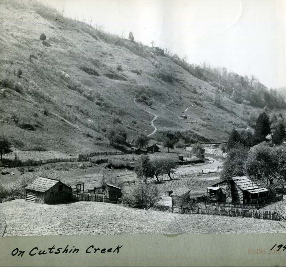
“On Cutshin Creek 1948.” Distant view of cabins, creek, hillside.[nace_II_album_022.jpg] [Photo not part of original Giffin research]
TAGS: Roscoe Giffin, People of the Pine Mountain School District, Harlan County, Kentucky, Appalachia, populations of Appalachia, education, Harlan County Schools, mountaineers, statistics of Eastern Kentucky,
ROSCOE GIFFIN
PEOPLE OF THE PINE MOUNTAIN SCHOOL DISTRICT, HARLAN COUNTY, KENTUCKY
A Study of Selected Aspects of Their
Population, Families, Economy, Social Organization,
and Values and Attitudes
as of
Summer, 1950
by
Roscoe Giffin
Berea College
TRANSCRIPTION PART 1 of 4 (001-050)
INTRODUCTION
This study has its origin In the relation which is developed between Berea College and Pine Mountain Settlement School since 1949. The history of this development is not known in its entirety to this writer and the details are not of importance to this statement. Perhaps it is enough to say that a relationship of mutual aid and of partially overlapping boards has been created such that certain of the resources of each are of benefit to the other. As one phase of this exchange, the staff of Berea College has been called on from time to time to serve an advisory and research capacities. On problems of the Pine Mountain School. It is a specific aspect of this general relation, which has prompted this study.
The specific conditions which gave rise to this study are approximately as follows. In 1949 Pine Mountain school;s boarding high school program was discontinued, and it became a part of Harlan County’s elementary school system. Five district schools in the adjacent area were closed and consolidated into the one school at Pine Mountain. Since the school would now be much more closely related to the population of the area than had been true during the recent years of the boarding high school, the administration, both a Berea College and the Pine Mountain School, were of the belief that a socio-economic survey of the area would be of value in providing a “set of benchmarks” with which future changes might be compared and the influence of the new school program, perhaps, measured.
Another factor prompting the obtaining of the data of this study was the information that a major coal mining development was planned for the near future relatively close to Pine Mountain School. A study of the area …….
p. 002
………………. before this change would thus provide not only a basis for future changes, but might reveal some of the resources of the area which would be useful in coping with the problems which a new mining venture would create. However, this writer [Giffin] was unable to uncover any factual basis for this new development. A development of almost as much importance, however, as a new mine, has been the construction of a new highway running from Big Laurel a few miles below Pine Mountain School on Greasy Creek, over the hills into Perry County, to the Leatherwood Mine of the Blue Diamond Coal Company. This latter [mine] is a tremendous mining operation whose influenced by way of employment was important to the Pine Mountain School area well before the road was opened. The new road, plus highway improvements elsewhere in the area, will magnify considerably the significance of this mining enterprise. We will have more to say on this subject in the concluding section when we engage in a bit of prognostication.
Just in case someone should read this document who has not been to Pine Mountain School, we will briefly describe some of the locational and geographical characteristics of the school. The school takes its name from the extensive, sharply ridged mountains called Pine Mountain, which runs in a north east- southwest direction throughout Harlan County and beyond, rising some 1000 feet from the valleys on either side. It’s been a major barrier in Harlan County, as evidence, politically, economically, socially and almost any other way one can imagine. It was not until the mid-1930s that a road was constructed across the mountain.
Valleys of the area are characteristically narrow and drained by creeks which form the headwaters of the Kentucky River system. Flatland for farming is rather scarce as a consequence. Cultivation was pushed …
p. 003
…………… up the hillsides as the population expanded during the past century. Since the region is the beneficiary of rather high annual rainfall ranging between 40 and 50 inches, with a growing season of nearly six months, the hillsides have produced great stands of timber. Even though there is left but little virgin timber, lumbering a more recent growth and of species formally undesired, is an important source of employment.
As is well known, this general region of southeastern Kentucky has become an important coal producing region in the past 30 years in it’s reserves and possibilities for further operations are immense. However, at present, competition with other energy fuels confronts the mining industry with a serious problem of maintaining full production and employment.
In order to acquaint the reader with the location of the various neighborhoods in school districts which have been consolidated, their location will now be briefly considered. Approach Pine Mountain School from the West after turning off of US 421. Just before it begins the assent over Pine Mountain and down to Harlan, we travel along a winding, graveled road, which, after several miles, brings us to the break of Laurel, the western limit of the Incline School district. In the summer of 1950 this district contained some twenty one houses scattered along perhaps four miles of the valley. The name. “Incline” arises from the fact that there used to be a power operated incline [railroad] in the region which was used to haul logs up and over Pine Mountain.
Although the legal boundaries of the Incline school district are sharply separated from those of the next one, [called] Divide, the neighborhoods as identified by the residents, change only gradually, and thus create a border area of uncertainty. But since this is a common characteristic of….
p.004
…………. the delineation of social areas it is nothing specific to this region. Twenty-five homes are scattered along this road to approximately the point where it intersects with the new road coming over Pine Mountain from the south.
Here begins the western limits of the Pine Mountain neighborhood and school district. It extends along the mountain until it merges with the Isaacs Creek neighborhood. However, a part of the old Pine Mountain District extends for perhaps a mile down the Greasy Creek canyon [valley] which breaks away to the northwest from the Pine Mountain, at the location of the Settlement School. Exclusive of the residences on the school grounds, and those occupied by employees of the school, there are nine homes in the neighborhood.
The Isaacs Creek area continues along the mountain to the east, to the Letcher County line. Settlement is limited, particularly in the upper limits of the neighborhood, by the uneven and hilly topography, so that there are but nine households.
If we now reverse our journey and proceed to a point, perhaps two miles west of the settlement school, we find a road turning sharply to the right, climbing up and over a hill and then dropping sharply into a narrow valley called “Gabes Branch”. Until several years ago, this [area] was one of the few remaining stands of Virgin Timber in the area. It is no longer such for several lumber companies have recently been in there cutting, and not on a sustained yield basis. At the intersection of this creek and another several miles below the crest of the hill are located three homes. At almost the upper limit of the unnamed creek, previously referred to as “another”, is one more home. The last occupied house in a valley which contains two or three vacated houses.
p. 005
Returning now on our journey and taking the left fork of the road just before the bridge across Greasy Creek, near the Settlement School, we proceed about a mile and 1/2 to the Little Laurel neighborhood. This area extends both ways along Greasy Creek at its junction, with the Little Laurel Creek which flows into it from the east and up the latter Creek itself. If we head up little Laurel Creek, either in a sturdy truck, Jeep or on foot, we finally encounter a few homes scattered along this remote, but very beautiful valley. We identified 17 houses as being in this neighborhood.
The next area we encounter along the downward course of Greasy is that of Big Laurel. Most of the houses in this neighborhood are concentrated either at the joining of Greasy and Big Laurel Creeks or along the lower reaches of the latter creek. There are 26 houses in the Big Laurel neighborhood. The most populous of the eight neighborhoods in this study, and the nearest approach in the region to a “community”. The Big Laurel Creek flows from the east out of the area known as “Turkey Fork”, whose limits are the hill summits along which runs the Perry County line. The Turkey Fork School District was not included in the Pine Mountain consolidated school district at the time of this study, due to the road being so poor that the busses could not get into it and being too far for most of the children to walk to the bus. However, in the past year, the school has been closed and consolidated.
Below the Big Laurel settlement and continuing along Greasy toward the Leslie County line is a neighborhood finally identified as “Greasy” [the same as the Creek]. Only seven families reside here, although the actual social limits of the neighborhood probably include additional houses. Since they would be in Leslie County, they are not considered in this study.
p. 006
SUMMARY AND CONCLUSIONS
In recognition of the fact that the major value of this study will be that of a reference work for future comparison, we shall first present a summary of the principal findings. An effort has been made to present these remarks in as non-technical a manner as possible. Any reader interested in the statistical details and more elaborate description is, of course, referred to the main body of the document.
Population: Growth and Composition: The population of the Pine Mountain School District as of mid-summer, of 1950 was approximately 631 which represented around a tenfold growth. From the estimate for 1870 of 60, the earliest date for which we have any reliable indications. The present population is one which must be called “young” in comparison with the U. S as a whole: Fifty six percent were of the ages 19 and under, as compared to 34% for the entire US as of 1940. females exceeded males by a ratio of 84 to 100. Although our data do not lend themselves to the computation of birth rates, it is evident from other information that the reproductive powers of this population are matched by few other areas of the U. S. The 114 married women of the area who have borne children have 549 living an average of 4.8. Some of our evidence points to the conclusion that the birth rate at present is about the same as for the past 50 years.
The formal educational opportunities of these people have been notably scarce. Perhaps, it should be added that the demand for such education has also been quite scarce. Whatever the reason, we find that only about 1/4 of those age 18 and over have any schooling beyond the 8th grade.
p. 007
The occupation and location of this population place it in the census category of “rural non-farm” for, although it is definitely rural, farming was the chief source of livelihood of less than 10% of the families. Lumbering was first by a large margin. Coal mining second . Followed in order by farming. construction, and distribution. As a source of income, [1950] public assistance was of more importance than farming.
Any expanding population is confronted with the problem of increasing its resources for living. During the early years of settlement, this was readily done by opening up new lands in the valleys and then later turning to hillside cultivation. But this populations continued to grow employment along other avenues, such as those found at present, was necessary. However, such adjustments have not been sufficient and as a result, many persons have chosen to migrate. Of the 213 children no longer living in their parental homes in 1950, only 61 were definitely known to be living in the Pine Mountain area. It. was interesting and surprising to discover that of those who remained at home almost 2/3 had received some education beyond the 9th grade as compared to but 1/3 of those who had migrated. Contrary to the publicity given in recent years to the migration of Kentuckians into other states, we found only 18 of these children who had gone to other states. Most chose to remain in Harlan or other adjacent counties.
Families. The information we have to offer regarding the families has little to do with the interesting dynamics and role patterns, which we know to be present in this area. We have been limited to more………
p. 008
……….. mundane aspects of the statistics of size and type. However, it is not an uninteresting fact to discover that nearly one – half of the 631 people residing in the area lived in the 35 households having seven or more members. There were about 121 households in the entire area. The median household contained the statistically possible, but actually impossible number, of 5.34 persons. We found only 19 homes with no children.
Income. The cash income distribution among these families presents a picture in marked contrast to that for the general U.S. population for the average is considerably lower and a larger proportion occur in the lower income ranges. 50 percent of the households had incomes in the year preceding our survey of less than $1725. But even within this area, we find considerable variation among the neighborhoods. Ranging from a median of over $2300 for Pine Mountain to $750 in Greasy Creek. An important addition to cash income is home production. It is difficult, if not impossible, to compute such a figure; But our estimates indicate a median value of $755 for such production. Generally speaking, the families of relatively high cash income were also those of [a] relatively high value of home production.
In an effort to determine some of the factors causally associated with the variations in income, we made a number of comparative relation analyses. The value of home production was studied in conjunction with land holdings and usages, ownership of livestock and equipment and in the households labor supply. In this region of narrow valleys and sharply sloping hillsides, there is no reason to expect to find that over 50 % of the households cultivated five acres or less, and only seven reported more than 10 acres in crops. For the entire area, we ….
p. 009
……..estimate approximately 450 acres in cultivation. When variations in acres cultivated were related to variations in the value of home production, a definite association is observable. But the correlation must be quite small. The general picture of land holdings is that of a high degree of ownership of very small scale operations. The gross comparison of size of household in home production without any refinements for the age , health and other variants among the households Indicated a fairly clear relation, such that the two series increase together. The preceding comparisons with the variations in value of home production have been the measures of land and labor. If we turn now to such indices of capital as the ownership of livestock, with hogs as a specific case, we find evidence of a positive relation as one would expect. The comparisons we have prepared are all of a relatively low degree of correlation, and we must acknowledge that there are factors, perhaps, of greater importance, which we have not considered in this analysis of variations in home production. The most important are probably the most elusive and the most obvious are probably the least important. Probably the controlling factors are those very real, but hard-to measure items of attitudes, values, knowledge, family solidarity and morale.
Cash income variations were studied in relation to variations in occupation, age and the ownership of a car or truck. The. last mentioned, we recognize is perhaps an obscure connection which we shall try to make more obvious since the dominant employments were those of lumbering and coal mining. It is to these categories we must look for much of the explanation of cash income differences. Of the 66 households reporting cash income between $600 and $2500, 39 were found….
p. 010
In these two employments of mining and lumbering. Each of these employments, yielded an average for the year studied, which was noticeably in excess of the average for all the cases. Those. employed in mining reported average earnings just under $2500. Although over half were actually below this figure. Several cases of proprietors of mines were included and thereby raised the average somewhat age. of the hit of the house is a well known factor in determining the amount of cash income. The lowest levels of income were dominated by elderly persons of a median of 66 [years]. Yet, the highest income level was held by the next oldest group with a median of 52.5 [years]. The other income levels fell between these two extremes.; The median age of 40 for those in the $1500 to $2500 level was the lowest among the income classes. In an economy in which increasing reliance is being placed on wage jobs as a means of sustenance in which is essentially rural, non-farm ownership of a car or truck is obviously important. Consequently, we find that although those with earnings in excess of $1500 were 58.5 per cent of the households, they own. 73.3% of the cars and trucks. The higher levels of income are obviously both a result and a cause of the mobility made possible through the ownership of a vehicle.
The extent to which a family or population aggregate shares in its social and economic opportunities of its society is known as the “levels of living”. In order to develop a picture of the levels of living found among this population, we have made use of a measuring method which assigns various weights to the possession of certain….
p. 011
Material goods into several indicators of social participation. The results is known as a “socioeconomic status scale score”. The average score of 55.5 is noticeably lower. By from six to 16 points than the averages for Oklahoma, Louisiana and Kansas, as reported by the inventor of this scale. The statistically observed variations among the households. Corresponds with that impressed upon the writer in doing the field work for this study. Although he made no study of the actual consumption patterns of these people, further light can be cast upon variations in the level of living. By considering the distribution of consumers, capital goods. thus, for example, we find that of the. 31.4% of the households having cashing come in excessive $2500. 38.9% of them lived in painted frame houses as compared to 7.9% in unpainted. In general, we find that the higher income levels owned a larger proportion of the various consumer capital goods than was their actual numerical strength in the entire group of households. The level of living which can be achieved by the members of a family at a given level of cash and home produced income is obviously dependent upon the number of persons who must share in it. The generalization involved in the proceeding sentence was found to be true, with the exception that the two cases of 1 person households, had lower per capita incomes than the 2 person households. Which were found to have a per capita income of $721 the highest of any. all cases of nine or more persons were associated with per capita incomes of $200 or less.
Mobility: Residential and Occupational : We have made no effort to locate mobility studies of the population of other areas. So we are in no position to say whether these people are more or less mobile than …
p. 012
others. Thus we are limited rather strictly to factual reporting. For our analysis of residential mobility we have concentrated attention upon the 106 husband-wife pairs in the area and have considered them as to length of residence, number of places in which they have lived, and travel experience. In 87 cases out of the 96 for which we have information, husband and wife had lived approximately the same number of years in the area. In 56 cases, they had spent between 16 and 20 years out of the past 20 in the Pine Mountain area.
For a big majority of these couples, the place of residence has been quite stable during the past 20 years. For a population with such low incomes in possessing cars in less than half the households, it is not surprising that 37 couples indicated they had not traveled beyond the limits of the immediately adjacent counties.
Our effort to study occupational mobility was limited to the different types of occupations held by those who have been members of the labor force during any portion of the preceding 20 years in over. two thirds of the cases for which information was available. Two or less occupations were indicated the. lack of young men in the labor force is clearly shown by the fact that 64 of the 88 known cases had been in the labor force over 15 years.
Welfare provisions: All of the various forms of public welfare and assistance present in the General Society are to be found among this population, despite its smallness of size in rural location. Of the fifty seven cases located in the interviewing. 18 were for old age pensions and 15 for aid to dependent children. Payments in all these categories. Were generally low, with the exception of those for veterans who averaged over….
p. 013
$1000 due to the presence of several cases of high disability. In addition to the various forms of public aid, some security and assistance was being provided also by the households for 42 dependent persons well over half of these were married children and their children. Who had returned to live in the parental households in? only three cases where parents living in the households of their children.
Social organization and participation: The population groupings in addition to the immediate families to which we have given some attention are those of kinship, friendship, neighborhood and formal organization. Classes and trade center relations, which are usually not thought of as groups, were also considered as phases of the general social organization of the population.
Kinship. Ties are important, both for their frequency and their determination of visitation and mutual aid relations among the households. The. extent of the kinship ties is almost amazing, but we shall only sight. An example at this point by inquiring if the readers know of. any area of like population size in the US where one can find 40 families who are related to 5 and more other households by relationship of first cousin or closer.
Visitation patterns are indicative of the presence of an informal social system, serving the ends of pleasure and mutual aid as is to be expected from the comments above concerning the extent of family relationships. Most of the visitation is among kin. It seems probable that kinship is more important than geographical factors in determining visitation patterns. Visits between Ken, not in the same neighborhood. Are more common than visits between non can in the same neighborhood.
p.014
Various kinds of friendship clique in. clicks in mutual aid groups were of course present. Considerations of age, sex, class and locality Can be inferred as the principal controlling factors. The only quantitative data to which we can refer in this regard is that concerning informal visitations among the various householders. Although we have no standards of reference, it is impressive to this urban dweller. Rather accustomed to being left alone by and leaving alone. His neighbors define 77 cases who estimated they had each received upwards of 275 visitors in the preceding year.
Although kinship is probably more important than neighborhood as a basis for social iteration, it is nevertheless quite apparent that this particular geographical factor is significant in forming a population grouping. This conclusion is supported inductively by our evidence regarding visitation patterns and inferentially My other general knowledge. the various neighborhoods appear to be quite distinguishable, not by — just by — location and known identification, but because of marked social and economic characteristics. Details cannot be developed in this summary, so the reader will need to consult the text for supporting evidence in most. cases, the neighborhood seemed to possess a distinct “personality”. Which, at this stage, we sense intuitively, although the various factual items support the conclusion of differentiation, but without providing the means for outlining the sensed personality differences.
Formal organizations are almost conspicuous by their absence among these people. Four church groups, a Masonic Lodge, United Mine Workers Union, three post offices and four or five stores, a bad exhausts the list of groups. Which might be designated, “formal”. Among the women, there were no such organizations It is thus not at all surprising….
p. 015
……… to find His households made very low scores on the.”Chapin Social Participation” score Since it is based entirely on formal group participation. The most common score was zero.
Social class can most easily be defined as a grouping of equals who interact more among themselves than any other persons. Equals refers to approximate similarity of economic and social opportunities, as indicated by income consumption, race, education, Etcetera. Although this was not a major object of the study originally, we have sought to show that there are at least three rather distinct segments in the population which might be thought of as lower, middle and upper classes. Our supporting evidence involves a ” socio-economic status scale score”, Cash and home produced income, occupation, and land occupancy as to size and tenure status.. All of these appear to point to the indicated distinct groupings. in sociological terms, the important consideration of course, is whether or not such evidence roughly outlines the limits. Of interaction sets so that we can say that the lower class people interact more within their own class membership than outside it. And likewise, for the other classes, we have. no direct evidence to contribute on this point. But the findings of other studies show that the various socio-economic measures are closely associated with interaction patterns.
The extent to which rural people are associated with urban residents in a community sense is discernible through a study of trade center relations. As self sufficiency has been replaced by interdependency among urban as well as rural people, buying and selling religious and educational and other relations have developed. Which link urban and rural dwellers in a web of mutual dependencies in the area of our study. These relations have been slow to develop and …
p. 016
Are at present determined almost entirely by job and buying requirements for the. population as a whole trips to Harlan (a distance of about 18 miles) are relatively infrequent: Approximately a third of the men and women from whom information was obtained went to Harlan on business trips, an average of 1 to three times per month.
Values and Attitudes: Social science is becoming increasingly concerned with question of the attitudes which people expressed toward various aspects of their life, and with the values or reasons which. Underlie these attitude – expressions. As one seeks to describe such items, he quickly finds himself drawn in the direction of trying to formulate a statement about the way in which the values are organized and their core or central theme. This is perhaps just another way of saying.” philosophy of life”, But we shall avoid the particular phrase because our study is much too limited to justify this attempt. Our efforts were limited in the field work to inquiries about attitudes. And values related to the area as a place to live. The quality of the land for farming. Desires of parents regarding a residence place and education of their children, employment for their children, extent of acceptance of labor unions and the satisfaction with the new consolidated school arrangements. In addition to the statistical description of these items, we have entered into some speculative assertions concerning some of the values or reasons associated with other rather obvious patterns in the culture. We have then leaped even further beyond the limits of our data in an effort to show that the theology of the Appalachian area is a crucial matter in understanding and explaining the attitudes. Values and the general pattern of culture of these people.
p. 017
Despite all that this area lacks as measured against a rather urbanized point of view, The people we interviewed were generally closely attached to the location. 2 thirds of them stated it was either a.”” pretty good” or ” very good.” place to live.’ the same proportion had no intentions of moving away. The reasons expressed to justify these attitudes indicated that such forms of “income” As peace and quiet, the presence of many relatives and friends and home ownership were of more importance than the disadvantages of the low quality of the land and various other inconveniences.
Some evidence of the strong bonds of family affection is shown by the parent’s desire for their children ” to live around here.”. This was the most commonly expressed desire regarding the residence location of their children, although it was balanced by various other statements pointing toward recognition that they would be better off elsewhere. in view of this possessive attitude, it was something of a surprise to find that 40% of the parents wanted a college education for their children. [a1] A cross tabulation of these two attitude groupings showed that about half those parents who wanted a college education for their children also wanted the contradictory value of having the children live near by. At present, there is but one college graduate among the population not residing on the Pine Mountain campus.
Those types of industrial employment with which these people have had most direct contact were found also to be the type parents wanted their children to stay away from. Coal mining took the honors for being most undesirable and timber work was second. Another attitude which stems from their direct experiences with one manifestation of industrialism, is that towards unions. This writer would hazard the….
p. 18
Guess that not even in an industrial city would one find such overwhelming support of labor unions as these people expressed. Of those expressing an opinion, Six were in favor of labor unions for every one disapproving.
The consolidation of the district schools met with a high degree of acceptance in its first year of operation. We found less than 10 per cent responding “no” to the question: “Was the school as good as those of other years?” The hot lunch program was unanimously approved, although it had monetary costs to budgets undoubtedly straining under the demands of large families.
There are any number of items of the patterned behavior of these people. just as among any other population which present an interesting challenge to him who seeks the explanation or meaning of the behavior. We have attempted this in a limited number of cases. With the recognition that, in many cases, other explanations might be equally valid, since the. statements are already presented in a condensed form, we will not present any summary at this point.
Our interest in relating the theological and religious presuppositions of these people to other aspects of their culture has grown from the conviction that knowledge of the resources, population and social organization was insufficient as an explanation of their way of life, that there was a missing factor in the equation. Somewhere in the study of a culture, one will generally find some clues which express what the population considers to be important, that “what oughts” of life. And certainly in the Western World, religion has been a major locus of such directives.
To illustrate the general ideas expressed in the previous paragraph, let the reader recall from earlier comments in this summary, or …
p. 19
From his own knowledge of the economic characteristics of the area, particularly as regards the level of living. Then let him bring to mind some of his own mental images of the levels of living which have been achieved by other people in areas having similar natural resources features. Various parts of New England and Pennsylvania. Some of the regions of Central Europe will serve the case. These. have been areas which in many instances have been the scene Of considerably higher levels of material well being, as well as noteworthy achievements in the intellectual and esthetic fields. What explains the difference?
Such studies are available on the religion of Southern Mountain people, [and] point to the conclusion that it is salvation centered and ” other worldly” In its premises. since Heaven is the individual’s ultimate home, and since the end of the world is soon at hand, the hardships of this earth are to be accepted. And poverty may be exalted into a virtue. This particular. this particular religious manifestation has been shown by Richard Neber to be common among the religions of the disinherited The question may certainly be raised as to whether or not such views are rationalizations, after the facts of life. However, there is no doubt that a religion of the Millennium will most certainly reinforce and preserve the material shortcomings of present day existence.
p. 20
POPULATION GROWTH AND COMPOSITION
The population of the area understudy was very close to 631 during the Midsummer of 1950. We have previously indicated that the area of our survey included the five school districts which. Had been consolidated into the one school at Pine Mountain Settlement School. All households in this area were included, except those whose major occupational attachment was to the settlement school. We made an effort to include in our data those who happened to be away from the area at the time by relying on secondary sources of information. We believe the total count is within 1% to 2% of the true but unknown figure.
Population Growth: Early settlement of this region appears to have been shortly before the Civil War. Because of the probable impossibility of obtaining the census count. for this specific area, even. though we were to journey to Washington DC, we have tried to develop some approximation which would help us to get at least a rough idea of the population growth since the period of settlement [in the area]. The method we have used was that of rather lengthy interviews with a number of the oldest residents of this area as to ” What families were living where and when” From this inquiry, it appears that in 1870 the population of the area included in our survey Was about 60 persons? By 1900 the populace approximated 150 to 200 persons. On the basis of our figure of 631 for mid-1950 we see that there has been approximately a tenfold growth in the past 80 years.
Area and Sex Distribution: To those concerned with the planning of institutions and social organizations which must Make future commitments and investments of varying magnitude. The age and sex distribution of the population with which they are associated is of major importance. One example….
p. 021
… Of the significance of such considerations is that the future demand for the services of an institution may be closely related to the age or sex structure of the populace. And to meet a changing demand, facilities of supply may need to be prepared or planned for years in advance.
In Table 1 Is shown the age and sex distribution of the population we have studied, both in numerical and percentage form. To aid the reader, to readily see the agent sex characteristics of the population we have prepared Chart 1 Which is known as a ” population pyramid”. In percentage Form. It graphically depicts the characteristics here under consideration Since the major outlines of the data are quite obvious when thus presented, We shall limit our verbal comments to a brief analysis.
The age distribution offers interesting possibilities for speculation and some very real and serious problems of public policy For the ages 19 and under, we had a population of 352 which represents approximately 56 per cent of the total population. By any standard, this would be defined as a “young population”. Let us compare, for example, the picture for the U. S as a whole in 1940 the last year for which we have readily available data. [1.] ; That year, 34.4% of the populace was 19 or less. In rural non-farm areas, the figure was 36.9; and in rural farm, it was 42.7. Obviously, this is a non-typical situation. And even within the general area of which Pine Mountain is apart, the percentage in these. age brackets is above the average. The percentage for the Cumberland Plateau region of Eastern Kentucky is 52.5 per cent. [2.]
- Sixteenth Census of the United States, Population, United States Summary, Washington, D.C. 1943. Table 7.
- Peers, H.W.. Age Structure of Kentucky Population. A.H.S. Bulletin No. 465. June 1944, University of Kentucky, Lexington, p. 34.
p. 022
TABLE I
AGE AND SEX DISTRIBUTIONOF THE POPULATION
[link address of table]
p. 023
CHART I
AGE AND SEX COMPOSITION OF THE POPULATION,
PINE MOUNTAIN AREA 1950
[link address of the chart]
p. 024
In the Cumberland Plateau region of eastern Kentucky, the percentage of person 60 years of age and older is noticeably less than that for the U. S as a whole: [2.] 5.3% as compared to 10,5%. Each group represents approximately 6.8% of the total population around Pine Mountain.
In those ages, generally considered to be the most productive years. 20 to 60, we find 35.6 per cent present in the Pine Mountain area as of 1940. Among the general population of the U.S. 55 .1 per cent were between the ages of 20 and 60. [3.] We shall leave it to the reader, at least for now, to speculate on the social significance of this aspect of the population structure.
In the total population, women outnumbered men considerably as measured by a man to woman ratio of 84 per 100. The. reader will note from TABLE 1. that until the 40 – 44 age level is reached. There were fewer males than females, with the exception of 25 – 29. Only between 20 and 60 was there. any excess of males. beyond 60. The total number of females was 25 as compared to 18 males. Whether the causes b. biological or socioeconomic, the consequences are nevertheless serious.
Reproduction Analysis: It is generally quite well known that reproductive rates, if not the powers, of the people of the Southern Appalachians are considerably greater than that of the nation as a whole. Whatever may be the forces at work to produce this situation, they are operative with considerable efficiency among the people in this study.
Data concerning the distribution of mothers, according to their age, in mid 1950 and the number of children ever born to them, whether at home, away, or deceased, are shown in TABLE 2, whether or not one could show….
- Peers
- Sixteenth Census of the United States, Ibid.
- Op. Cit.
p. 025
TABLE 2
MARRIED WOMEN BY AGE AND BY NUMBER OF CHILDREN EVER BORN PER MOTHER
TOTAL CHILDREN EVER BORN
[insert link]
p. 026
From a careful analysis of these data in some.”free-hand extrapolating,” That the younger women will produce fewer total children than the older is beyond the writer’s powers. However, it is evident that if the women yet in childbearing ages under 45 usually bear as many children as have those beyond this age, there will be further expansion of population in this part of Kentucky.
One bit of information on which we want to consider for a moment emerges at the extreme lower right hand corner of TABLE 2. Here we find the figure of 631 as indicating The total number of children ever borne to these women. If we include only those women who have borne children, we find the average number of births to be 5.5. If we subtract from the 6. Thirty one bursts the 82 who were still born or have died since birth, we find that these 114 women have 549 living children, an average of 4.8.
We have sought in another way to obtain some information on which would enable us to throw some light on the question of whether or not the birth rate is decreasing among these people as Interview we had asked for the number of children in the MOTHERS 45 AND OVER AND THEIR OWN MOTHERS COMPARED AS TO NUMBER OF CHILDREN EVER BORN PER MOTHER AND AS TO TOTAL NUMBER OF CHILDREN EVER BORN miles from which the husband and wife, or either alone, as the case may be, had come. We have prepared TABLE 3 in order to compare the data on present day families with those of this earlier generation since we have assumed, and probably incorrectly so in a few cases. that all of the mothers of the husbands and wives interviewed, were beyond the childbearing [age]. We have included in this table only present mothers over 44 years of age. By so doing, We have sought to compare only cases of women beyond the usual age of childbearing, or women whose families may be considered completed.
If we compare the average number of children born to those mothers over 44 who were interviewed, with the number born to their mothers, we find a….
p. 027
TABLE 3
MOTHERS 45 AND OVER AND THEIR OWN MOTHERS COMPARED AS TO NUMBER OF CHILDREN EVER BORN PER MOTHER AND AS TO TOTAL NUMBER OF CHILDREN EVER BORN
[insert TABLE]
Handwritten note at bottom of Table:: “Their Mothers” Their children will be [?] by [?] of sisters among “…45 and over…”
p. 028
… close similarity. Average among mothers interviewed is 7.56 as compared to 7.67 among their own mothers. Another way of comparing these two groupings is on the basis of the total number. Of children born to the two categories of mothers. The total among the present group is 295; For their mothers, the estimate is 299. [1] The writer makes no pretense to being a population analyst, but these data appear to him to indicate that for the span of time involved in these two groupings, the birth rate was approximately a constant.
Educational Status: For purposes of this analysis, we are dividing the population into two segments of those 18 years of age and over, and those less than 18 but at least six. For the younger group, we have classified them by age and highest grade achieved. These data are presented in table 4. The writer must admit that the table is so full of figures that it is even confusing to him. The presentation is made here in this form for the sake of completeness Without entering into a lengthy statistical analysis of them, we shall offer only a few comments which is hoped will aid in the interpretation.
First of all, the reader’s attention is called to the number of persons at. each age level. as shown in extreme right column of the table, The point of emphasis is the similarity in the magnitude of the numbers from year to year. Then so that we may get the contrast regarding educational status. The reader is asked to consider the totals along the bottom of table 4 for each grade in school. The point to emphasize here is that though the totals are quite variable among the grades from 1 through 6 they do hover around an average which would run through approximately 25.
1, We have not used the number of children as given in the father’s family in these comparisons, because the results did not agree with what might be called our “common sense”. The average number of children indicated in this category was 9.6. as compared to the 7.67 among mothers. There is no logical reason why this should be so. Further, since most of our interviews were with women, the chances of accuracy seem greater for their own parental families than for those of their husband.
p. 029
TABLE 4
EDUCATIONAL STATUS OF YOUTH, 6 – 17 YEARS OF AGE
[insert link]
p. 030
TABLE 4 (PAGE 2)
EDUCATIONAL STATUS OF YOUTH, 6 – 17 YEARS OF AGE (page 2)
[insert link]
p. 031
But the number who have gone as far as the 7th and 8th grade. drops sharply when compared to the 6th and earlier. From then on, through the 12th the numbers fall rapidly. Yet, as stated above, the numbers in each age level are considerably more stable.
Just from looking at the arrangement of the data in this table, it is quite evident that a large number of children are behind the grade, which is usually associated with the various ages. To the teaching staff. This lack of correspondence between ages and grades is of considerable significance. For it presents them with the task of offering the same educational diet to children differing sharply at times. In their physical development. To the older students also, it may present an unpleasant situation which may have the final consequence of causing him to leave school entirely.
The statistics for the educational status of those 18 and over is presented in TABLE 5 but without the detail given in the table for those under 18. The general story which these data have to tell us is one that is rather well known. That rural people have fewer educational opportunities and perhaps fewer reasons to seek it than urban people is well known. And that this applies with particular vigor to the people of the South is also common knowledge. Thus, we find in this population but 56 persons who have had any schooling between the 9th and 12th grades, 37 of of whom were women. Seventeen have had some college or technical school, although only one is a college graduate. Of the total of 299 in this age category, 73 per cent have completed the 8th grade or less.
p. 032
TABLE 5
EDUCATIONAL STATUS OF MEN AND WOMEN 18 YEARS AND OVER
p. 033
Occupational Distribution: Mary and the analysis of the composition of a population to include occupations as one of the topics. We have chosen in this study, however, to reserve the more detailed consideration of this subject to a section entitled. “Variables Associated with Income”. Interest there focuses on occupation as a determinant of variation in the cash income of the various households. But because occupations are a significant phase of composition, we shall present our findings in as a summary manner at this point.
Among the heads of the 121 households studied, the major occupations defined as chief source of cash income – Were as follows in rank order of numerical occurrences: Lumbering, coal mining, farming, construction, and distribution. A variety of other. employments were included in a catch all of “all others”. Retired and unemployed persons formed another category.
Lumbering and coal mining accounted for 50% of the total. The fact that mining was but half is important as lumbering as a source of employment reflects the distance in difficulties of getting from this region to the mines, as well as the presence of a major lumbering operation on Gabe’s branch. In the summer of 1950. A ” conversational survey” With several well-informed persons in the summer of 1951 Indicated that the employment pattern was much the same, although the lumbering operations were much further removed, and the road to the Blue Diamond Coal Mine was nearly completed.
In the areas of seemingly remote from urban influences, it was a considerable surprise to this investigator. to discover the very limited importance of farming. One is accustomed to thinking of farming as….
p. 034
…. Being the occupation of those who live in the country. but less than 10 per cent claim this to be the major source of their cash earnings. In view of the small amount of land under cultivation in relation to the population size, this low level of significance of farming is not surprising. [1]
Marital Status: Another topic customarily considered as a phase of the study of population composition is that of the marital status, usually in relation to the age and sex distribution. The raw data for this analysis are available. but we have not done the necessary tabulations up to the time of this writing. However, from other bits of related information, it is possible to put part of this picture together.
Although it is common to learn of persons in the mountain area marrying at an early age [2], we found but two persons under 20 who were married, We will thus use 20 as our age criteria for this analysis, for it will then facilitate comparison with the U.S. Census publications.
The computations necessary to obtain these data are presented as follows in TABLE 6.
1.See TABLE 19 and page 65 for discussion on and data regarding agricultural land.
2. The “marryin” age for girls is sometimes spoken of as 16.
TABLE 6
COMPUTATIONS REGARDING MARITAL STATUS
| ITEM | MALE | FEMALE | TOTAL |
| Population 20 and over | 138 | 141 | 279 |
| Persons in husband-wife pairs | 106 | 106 | 212 |
| Nonmarried: widowed, divorced, or never married | 32 | 35 | 67 |
| Known widowed or divorced | 3 | 15 | 18 |
| Balance never married | 29 | 20 | 49 |
p. 035
The percentage of persons who were married as of 1950 was seventy six: For males and females respectively, the figure was 77 and 75. in comparison with the 1940 US Census data, we find this is generally a higher percentage of. married persons than for the US as a whole and in various categories of the percent of married females in the Pine Mountain area in 1950 was 1.4 percentage points less than that of females in rural farm areas in 1940.[ 1] Otherwise, the percentages for men and women are in excess of the U. S averages for urban, rural farm and rural non farm. [2]
Population Adjustment and Balance: Earlier in this treatment of population, the significant growth in the area during the past 75 years was considered. In response to its own growth a population is continually faced with striking a new balance with its resources or opportunities for living. Confronted with this problem, Thomas Malthus concluded long ago that populations tend to multiply up to the maximum carrying capacity of the land, so that the balance tends to develop at the subsistence level as the population approaches this maximum. Various checks come into play as such as the positive ones which raise the death rate and the negative checks which reduce the birth rate.
A further method for immediately disposing of surplus numbers, and one to which Malthus seems not to have given much weight, is that of immigration. It is to this adjustment of the Pine Mountain population that we will attend principally in this section.
- Carl Taylor, et al, Rural. Life in the United States. N.Y, Knopf, 1950., p. 228.
- The comparisons with 1950 census data may show a reduction of this difference. Such 1950 data as the rider has available. Show that for the 14 and over age group, there was an increase of about 28% for males and 24 per cent for females, as compared to 1940 for the entire US population. Source: 1950 Census of Population, Preliminary Reports, February 25, 1951, Series PC,- 7. No 1. U.S .Department of Commerce Bureau of the Census.
p. 036
During the early years of the settlement of this area, there was sufficient food and other resources available, so that the expansion of families could be absorbed within the area This was taken care of at first by the settlement of new lands. But then, more recently, by the division of the originally large farms among the heirs. Throughout the mountain country, there has been a progressive reduction in the size of farms, so that to day, many are too small to provide even a subsistence living. [1] In response to this situation, a population faces the. necessity of adjusting to a new balance through one of the following processes: Exporting some of its surplus members to less crowded regions; Reducing the plain of living; Developing new resources or reducing its birth rate.
We want to present shortly some of the data we have regarding the first form of adjustment in indicated, immigration. At a later point, we will want to comment in more detail upon the question of resource expansion, but for the moment it is enough to point out that the exploitation of timber and coal and their exchange for money are evidences of adjustment via the 3rd Avenue indicated with respect. to the adjustment through reduction in the plain of living, we have no available data, but this writer would speculate that this has been one method of adjustment The destruction of the natural food supplies such as Fish and Game, the apparent exhaustion of most of the hillside cornfields, the loss of nearly all handicraft skills seem hardly to have been balanced by the gains for public works. So wage jobs, as have been available, have been irregular and have provided a rather low annual income. The rider feels confident that the actual food….
[1.] Davis. D.H., The Geography of the Mountains of E.Kentucky , Frankfort, KY: Geological Survey, Geol. Reports, Series 6, V. 18, 1924.:
p. 037
…. Consumption as well as housing levels among those families which today have Sufficient land resources to be fairly self sufficient, exceed considerably that of those families who are entirely dependent upon the exchange economy. But it should be but it should be mentioned again that this is purely speculative and is not based on recorded data.
As regards the adjustment of population to opportunities for living through a reduction in the birth rate, we have already presented and interpreted data which appeared to indicate that, as yet, this process of adjustment has not become important It will be recalled, but a comparison of the number of children ever born to mothers over 44 with the number born to their mothers, was approximately the same. During the process of the interviewing, the writer sought to gain some impression from the younger married persons as to their norms of the “right number of children”. Although this was not a planned sample or census of such persons, there was a preponderance of opinion among those persons pointing to considerably smaller families than those from which they had come Thus, it is possible that in the future a reduction in the birth rate may figure as one method for achieving a more satisfactory balance between population and resources.
Our promise, of several pages back, to attend principally in this section to immigration as a method of adjustment, was somewhat forfeited to several other methods of adjustment and balance. But we shall turn directly at this point to the question of emigration, since we have certain items of information concerning both the emigrant and non-migrant population, we will handle this subject by means of comparison.
p. 038
TABLE 7
CHILDREN NO LONGER LIVING IN PARENTAL HOME BY SEX, INDUSTRIAL ATTACHMENT, LOCATION, AND FORMAL EDUCATION
p. 039
In order to compare the migrants from the area with those who have chosen to stay, we have prepared a rather complicated tabulation of all living children who are no longer residing in the parental households now established within the Pine Mountain School District. These children consist of those who no longer live within this district. Those who live within it, plus a small group for whom we did not obtain information as to location, but who have probably emigrated. Each member of these groups has been classified as to sex, formal education and industrial attachment. This four- way classification is shown in TABLE 7 Children No Longer Living in Parental Home by Sex, Industrial Attachment, Location, and Formal Education. since such a table is very useful for analytical and comparative purposes, but very difficult to read and discuss, we have placed several aspects of the data in separate tables, The complete table is included simply so that all of the data are available for anyone who desires to make other comparisons.
The first comparison we want to consider for this specific population is the distribution by location and sex, as shown in the following table.
TABLE 8
CHILDREN NO LONGER LIVING IN PARENTAL HOME BY LOCATION AND SEX: NUMERICAL AND PERCENTAGE DISTRIBUTION BY LOCATION.
| LOCATION | NUMERICAL | PERCENTAGE | ||||
| Sex | Sex | |||||
| Male | Female | Total | Male | Female | Total | |
| In P.M.S.D | 29 | 32 | 61 | 47.5 | 52.5 | 100.0 |
| Out of P.M.S.D | 53 | 78 | 131 | 40.5 | 59.5 | 100.0 |
| Unknown | 6 | 15 | 21 | 29.5 | 70.5 | 100.0 |
| TOTAL | 88 | 125 | 213 | 41.261 | 58.8 | 100.0 |
p. 040
The first item of significance to note is that here again, we find the sex ratio favoring the females considerably. Out of this total of 213, for whom we have information, there are 125 women to 88 men. A ratio of 1.42 or 142 per cent. When we consider the sex distribution according to location, we find a considerably higher rate of out-migration for women, than for men. Within the Pine Mountain School District, there is nearly an even balance. But if we assume the “unknown” are also out-migrants we find by further computation, not shown here, that over 60% of those who have left the area are women.
Determining the percentage distribution by location within each sex category, as shown in the following table, we further highlight the greater out-migration rate for women. In brief, we can say that of all the men, 1/3, have stayed within the district as compared to barely over 1/4 of the women.
TABLE 9
CHILDREN NO LONGER LIVING IN PARENTAL HOME BY LOCATION AND SEX: PERCENTAGE DISTRIBUTION BY SEX
| Male | Female | Total | |
| In P.M.S.D | 33.0 | 25.6 | 28.6 |
| Out of P.M. S.D. | 60.3 | 62.4 | 61.5 |
| Unknown | 6.7 | 12.0 | 9.9 |
| TOTAL | 100.0 | 100.0 | 100.0 |
The next characteristic of these groups. Which we wish to compare is that of location and industrial attachment. These data are shown in table 10 Children No Longer Living in Parental Home by Location. Industrial Attachment and Sex. Those who have chosen to remain within the district are employed dominantly, either in coal mining or lumbering, or are housewives.
p. 041
TABLE 10
LOCATION OF CHILDREN NO LONGER LIVING IN PARENTAL HOME
BY SPECIFIC LOCATION AND SEX
| LOCATION | SEX | |||
| Male | Female | Unknown | TOTALS | |
| Pine Mt. Area | 29 | 32 | 0 | 61 |
| Harlan County | 24 | 23 | 0 | 47 |
| Adjoining Counties | 9 | 13 | 0 | 22 |
| Kentucky Elsewhere | 5 | 7 | 0 | 12 |
| Other States | 5 | 13 | 0 | 18 |
| No Information | 6 | 15 | 4 | 25 |
| Non-Pine Mtn, Unknown | 10 | 22 | 0 | 32 |
| TOTALS | 88 | 125 | 4 | 217 |
p. 042
Among those who have left coal mining and lumbering [they] are of approximately the same importance as service in the construction – manufacturing categories. Marriage has claimed almost the same percentage of women among those who have stayed as compared to those who have left or are unknown.
A question which is continually arising is that of the educational achievements of those who migrate. The common sense knowledge, as well as various studies, have it that those who leave are usually those who have had the most formal education. [1] However, the information we have for this population indicates an opposite conclusion, as shown by an analysis of the data in TABLE 11. Children No Longer Living in Parental Home By Location and Formal Education. Numerical and Percentage Distribution by Location. These contrasts are pointed up, particularly by the percentage comparisons. Not much needs being said by way of description, since the data seem so clear on the general point. A surmising statement can be made by noting that of the out – migrants 33.5 % are in this categories 9 through 12 grades, some college, and trades as compared to 62.2% in the same categories for those who have remained within the District.
It is a well-known fact that the southern Appalachian area has been supplying other states and regions with a larger number of persons in recent years. Despite the high birth rates in this wider area, the population Has held about constant since 1940 due to migration. It is also common knowledge that Kentucky has exported a very large number of persons to the northern industrial states. Particularly Indiana, Michigan and Ohio. But here again, we are in for a surprise, so far as the people who have left the Pine Mountain School District are concerned. The general pattern of…..
- See Pail Landis. Rural Life in Process. McGraw- Hill , New York. 1948, pp.191 -198.
p. 043
TABLE 11
CHILDREN NO LONGER LIVING IN PARENTAL HOME BY LOCATION AND FORMAL EDUCATION, NUMERICAL AND PERCENTAGE DISTRIBUTION BY LOCATION [Link]
| Formal Education | Location | Percent | ||||||
| Out of P.M.S.D | Unknown | In P.M.S.D. | Totals | O | U | I | Total | |
| None | 9 | 2 | 0 | 11 | 6.9 | 9.5 | 0. | 5.2 |
| 1 – 4 | 19 | 2 | 4 | 25 | 14.5 | 9.5 | 6.6 | 11.7 |
| 5 – 8 | 51 | 6 | 7 | 64 | 39.0 | 28.6 | 11.4 | 30.2 |
| 9 – 12 | 28 | 7 | 33 | 66 | 21.4 | 33.2 | 54.0 | 31.9 |
| Some College | 15 | 0 | 11 | 26 | 11.4 | 0, | 18.2 | 12.2 |
| Trade | 1 | 0 | 0 | 1 | 0.7 | 0, | 0. | 0.6 |
| Unknown | 8 | 4 | 6 | 18 | 6.1 | 19.2 | 9.8 | 8.4 |
| Totals | 131 | 21 | 61 | 213 | 100.0 | 100.0 | 100.0 | 100.1 |
*Handwritten note at bottom of page: “Should this tabulation be included …..? ,,,,,is …..with usual pattern?
p. 044
Their migration has been to move elsewhere in Harlan County or into adjoining county. One of the population of 217 here under analysis., only 18 have gone outside of Kentucky. As shown in TABLE 12. Children No Longer Living in Parental Home by Specific Location and Sex. Harlan and adjoining counties have attracted 69. persons from our data, previously discussed, regarding industrial attachment. It may be inferred that marriage and employment in the coal and lumber industries have attracted a considerable portion of those who have gone to nearby areas. This follows also from the fact that coal and lumber are among the most important industries in this section of Kentucky.
These rather unusual patterns, with respect to the relation of migration to formal education and the concentration of the migrants within the same general region present us with a problem of explanation for which we lack satisfactory information upon a possible hypothesis might be somewhat as follows: Any expanding population which chooses to use migration as one of the adjustment techniques will be attracted in general to employment locations, which involve the least cost of travel from home and allow them to maintain more nearly intact family. And friendship contacts the pot. The population of this district has been expanding, and employment opportunities within Harlan County have been created by the expansion of its coal mining industry. In the past 30 years. To accept employment within the county would fulfill the requirements, as stated in our hypothesis above, develop. in coal and lumber in nearby counties, increase the possibility of fulfilling these conditions.
This does not, however, offer an explanation for the differentials in education as between the “Outs” and the “Ins”. Were our data in such a form as to permit a careful examination of the age distribution we might find…..
p. 045
TABLE 12
CHILDREN NO LONGER LIVING IN PARENTAL HOME BY LOCATION, INDUSTRIAL ATTACHMENT, AND SEX
| Industrial Attachment | Location | |||||||||||
| Out of P.M.S.D | In P.M.S.D | Unknown | Total | |||||||||
| M | F | M | F | M | F | M | F | |||||
| Coal Mining | 14 | 0 | 14 | 8 | 0 | 0 | 0 | 0 | 0 | 22 | 0 | 22 |
| Limbering | 10 | 1 | 11 | 15 | 0 | 15 | 2 | 0 | 2 | 27 | 1 | 28 |
| Distribution | 5 | 1 | 6 | 1 | 0 | 1 | 3 | 0 | 3 | 9 | 1 | 10 |
| Service | 6 | 8 | 14 | 1 | 1 | 2 | 0 | 0 | 0 | 7 | 9 | 16 |
| Construction & Manufacturing | 9 | 1 | 10 | 1 | 0 | 1 | 0 | 3 | 0 | 3 | 9 | 11 |
| Agriculture | 1 | 0 | 1 | 1 | 0 | 1 | 0 | 0 | 0 | 2 | 0 | 2 |
| BusineExec. & Professional | 1 | 6 | 7 | 0 | 1 | 1 | 0 | 0 | 0 | 1 | 7 | 8 |
| Housewife | 0 | 59 | 59 | 0 | 29 | 29 | 0 | 14 | 14 | 0 | 102 | 102 |
| Unknown | 6 | 2 | 8 | 2 | 1 | 3 | 1 | 1 | 2 | 9 | 4 | 13 |
| Miscellaneous | 1 | 0 | 1 | 0 | 0 | 0 | 0 | 0 | 0 | 1 | 0 | 1 |
| Total | 53 | 78 | 131 | 29 | 32 | 61 | 6 | 15 | 21 | 88 | 125 | 213 |
p. 046
…. some suggestions of an explanation. The implication here is that in recent years, employment opportunities in coal and lumber. Have probably not been expanding noticeably due to resource, exhaustion and competition of coal with other fuels. At the same time, education facilities may have been improving. Since employment opportunities were not expanding noticeably within the district, the younger persons who have perhaps more formal education have been migrating beyond the immediately adjacent counties. This suggests that the age distribution and distance of migration might be inversely correlated: The younger person in the migrating group have traveled a greater distance but at present, all of this is in the realm of conjecture. This is but part of an important research project which should be launched on the migration patterns of former southern Appalachian persons.
p. 047
FAMILIES BY SIZE AND TYPE
It is the purpose of this section of the study to describe and interpret our data. On the size and type of the family household units, as they exist in the socio-cultural setting. [1] the family unit is a social phenomena, a vast complexity, which offers as many sides for observation as the observer is equipped to see by virtue of skill and time available. This is but of sophisticated way of saying that when these data have been presented, there is yet left unstudied and unsaid many aspects of these 121 families.
It is a generally well known fact that Southern families produce more children than is characteristic of the rest of the United States. [2] And this is true of the families of the Appalachian region with even greater contrast. Thus it comes as no surprise to find our statistics for the families of this study supporting these generalizations.
one statistical measure of the size of these families is to compute that point on a scale of household size, which is exceeded by one-half. This value is known as the median and for the. 121 households of the study. It is. 5.34 persons and 50 per cent are less than this figure.
1. The term.” family” and “household” will be used interchangeably in all but three cases, the occupants of a household are genetically related and thus a family in the usual sense of the word.
2.: For a popular treatment of this subject sea. M.H.Verse, “The Child Reservoir of the South”, Harpers. Vol. 203, July, 1951, pp. 55-61. For a technical treatment of the data of several decades ago see: Howard W. Odum, Southern Regions of the United States, Chapel Hill: University of North Carolina Of less than this size. Press, 1936, p.474, 402. In 1940 all of the southern states were above the national level for the median size of household. (Dept. of Commerce Bureau of the Census, Statistical Abstract of the U,S,, 1950, p.50.)
p. 048
Another indication of the widespread distribution of children is that there are only 19 households in which there are no children at all.
Further emphasis can be given to this picture of household size by a slightly different organization of the data in which we compute the median for the population. Distributed according to the size of the household. For this computation, we obtain the value of 6.79. Thus, we can say that 50% of the people live in households in which there are more than 6.79 persons and 50 per cent live in the households of less than this size.
It is of some interest to study as regards size, only these households in which there are children. Of the total population of 631 for the area we find 588 living in the 102 households with children. The median household is just under six persons in this case. 5.82 Fifty per cent of this population live in households of seven persons and over.
One further measure of household and family size is that of the mode, the most common size. For those with children, the modal value is 3..88. and for all households, it is 3.52. Analysis of the households, according to the aggregate population, indicates a computed modal value of 5.58 for those with children and 5.55. for all.
Perhaps a note of conservatism Should be added to counteract what seems to be a common view concerning the preponderance of large families in the mountain areas. The most. satisfactory may be for the reader. To judge for himself in this matter is to consult table 13 where the basic data for this in the preceding statement in this section are presented. But the point can be made simply by stating that. There were only 35 households in which there were in excess of….
p. 049
TABLE 13
HOUSEHOLDS WITH AND WITHOUT CHILDREN AND THEIR AGGREGATE POPULATION DISTRIBUTED BY SIZE OF HOUSEHOLD
| HOUSEHOLD SIZE RANGE | ||||||
| WITH CHILDREN |
WITHOUT CHILDREN |
TOTAL | WITH CHILDREN |
WITHOUT CHILDREN |
TOTAL | |
| 1 | 0 | 2 | 2 | 0 | 2 | 2 |
| 2 | 2 | 13 | 15 | 4 | 26 | 30 |
| 3 | 20 | 1 | 21 | 60 | 3 | 63 |
| 4 | 15 | 1 | 16 | 60 | 4 | 64 |
| 5 | 17 | 2 | 19 | 85 | 10 | 95 |
| 6 | 15 | 13 | 75 | 78 | ||
| 7 | 12 | 12 | 84 | 84 | ||
| 8 | 7 | 7 | 56 | 56 | ||
| 9 | 7 | 7 | 63 | 63 | ||
| 10 | 5 | 5 | 50 | 50 | ||
| 11 | 3 | 3 | 53 | 33 | ||
| 12 | 0 | 0 | 0 | 0 | ||
| 13 | 1 | 1 | 13 | 13 | ||
| Total | 102 | 19 | 121 | 586 | 45 | 631 |
| Mean | 5.75 | 2.37 | 5.21 | 5.75 | 2.37 | 5,21 |
| Median | 5.82 | 2.50 | 5.34 | 7.07 | 2.79 | 6.79 |
| Mode | 3.88 | 2.33 | 3.62 | 5.56 | 2.60 | 5.55 |
p. 050
…. six persons. Only three had over ten persons. However, 47.5% of the 631 In the area resided within these 35 households of seven and more persons.
These households have been classified in a rather complex manner in terms of the various possible combinations based on the presence or absence of husband and wife, children and relatives or other non-related persons. The details are shown in TABLE 14 but it is perhaps sufficient to point out that 87 % of the households meet what might be termed the minimum “American standard family,” that of having at least a husband and wife present. Theories which had been broken by death, desertion or divorce constituted only 13 % of the total number.
However, the following evidence indicates that not all marriages of the children of these households fell into the groove of ” they lived happily ever after.” Eight married children with their six children were found living in the parental homes. Grandparents were providing for the care of all children whose parents were not present. In most cases, these broken marriages occurred among young people who migrated from the valley as a result of the various pressures and attractions let loose during the years of World War II.
END SECTION 1
GALLERY: ROSCOE GIFFIN – PEOPLE OF THE PINE MOUNTAIN SCHOOL DISTRICT, HARLAN COUNTY, KENTUCKY Part 1 (001-050)
-

- 001 giffin_1950_study_aspects_001
-

- 002 giffin_1950_study_aspects_002
-

- 003 giffin_1950_study_aspects_003
-

- 004 giffin_1950_study_aspects_004
-

- 005 giffin_1950_study_aspects_005
-

- 006 giffin_1950_study_aspects_006
-

- 007 giffin_1950_study_aspects_007
-

- 008 giffin_1950_study_aspects_008
-

- 009 giffin_1950_study_aspects_009
-

- 010 giffin_1950_study_aspects_010
-

- 011 giffin_1950_study_aspects_011
-

- 012 giffin_1950_study_aspects_012
-

- 013 giffin_1950_study_aspects_013
-

- 014 giffin_1950_study_aspects_014
-

- 015 giffin_1950_study_aspects_015
-

- 016 giffin_1950_study_aspects_016
-

- 017 giffin_1950_study_aspects_017
-

- 018 giffin_1950_study_aspects_018
-

- 019 giffin_1950_study_aspects_019
-

- 020 giffin_1950_study_aspects_020
-

- 021 giffin_1950_study_aspects_021
-

- TABLE 1 022 giffin_1950_study_aspects_022
-

- CHART I 023 giffin_1950_study_aspects_023
-

- 024 giffin_1950_study_aspects_024
-

- TABLE 2 025 giffin_1950_study_aspects_025
-

- 026 giffin_1950_study_aspects_026
-

- TABLE 3 027 giffin_1950_study_aspects_027
-

- 028 giffin_1950_study_aspects_028
-

- TABLE 4 029 giffin_1950_study_aspects_029
-

- TABLE 5 030 giffin_1950_study_aspects_030
-

- 031 giffin_1950_study_aspects_031
-

- TABLE 6 032 giffin_1950_study_aspects_032
-

- 033 giffin_1950_study_aspects_033
-

- TABLE 6 034 giffin_1950_study_aspects_034
-

- 035 giffin_1950_study_aspects_035
-

- 036 giffin_1950_study_aspects_036
-

- 037 giffin_1950_study_aspects_037
-

- TABLE 7 038 giffin_1950_study_aspects_038
-

- TABLE 8 039 giffin_1950_study_aspects_039
-

- TABLE 9 040 giffin_1950_study_aspects_040
-

- TABLE 10 041 giffin_1950_study_aspects_041
-

- 042 giffin_1950_study_aspects_042
-

- TABLE 11 043 giffin_1950_study_aspects_043
-

- 044 giffin_1950_study_aspects_044
-

- TABLE 12 045 giffin_1950_study_aspects_045
-

- 046 giffin_1950_study_aspects_046
-

- 047 giffin_1950_study_aspects_047
-

- 048 giffin_1950_study_aspects_048
-

- TABLE 13 049 giffin_1950_study_aspects_049
-

- 050 giffin_1950_study_aspects_050
TO CONTINUE, SEE
PUBLICATIONS RELATED 1950 Roscoe Giffin “People of the Pine Mountain School District, Harlan County, Kentucky” Part 2 (051-089)
PUBLICATIONS RELATED 1950 Roscoe Giffin “People of the Pine Mountain School District, Harlan County, Kentucky” Part 4 (130-157)
PUBLICATIONS RELATED 1954 Roscoe Giffin The Southern Mountaineer in Cincinnati Report – (in process)
PUBLICATIONS RELATED 1956 Roscoe Giffin From Cinder Hollow to Cincinnati 1956
Reprint for PMSS of Mountain Life & Work article – (in process)
SEE ALSO
ROSCOE GIFFIN Visitor – Biography
RETURN TO
PUBLICATIONS RELATED
VISITORS GUIDE to Consultants, Guests, Related Friends of PMSS